CoPaG and CoPaGAxs
Content
- General information on CoPaG
- CoPaG Concept - Relevance
- Classical plan networks (B,L)class and weak-forms
- Mathematical Concept and CoPaG Software
- Transformation Parameter Databases
- Transformation Parameter Accurcy Surfaces
- Download: CoPaG Manual (pdf, 1,1 MB)
General
COPAG realizes a strict 3D datum transition between a source system (S) and a target system (T) using the Molodenski approach. This is related to the geographical coordinates (B, L, h), so that identical points of differentdimensions (3D, 2D and 1D) can easily and simultaneously be used for the determination of a set of 7 parameters of a similarity transformation. The FEM concept of the COPAG software (fig. A) enables a robust L1 norm or a least squares estimation of an arbitrary number of 7 parameter sets in meshes, which are restricted to continuity along the borders of area meshes. The parameter sets and the mesh topology are stored on databases.
- CoPAG databases are used for the transformation of the plan positions (B,L) of a classical national network to an ITRF-related frame (e.g. ETRS89 in Europe)
- DFLBF databases are used in GNSS-positioning to transform the ITRF-related GNSS-position (B,L,h) to plan position (B,L) of the respective a classical datum, and for small meshes optionally to the standard height system H.
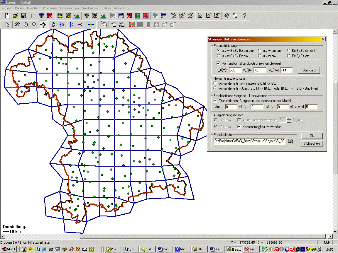
Figure A: ScreenShot of the CoPaG adjustmentsoftware (computation of CoPaG and DFLBF databases).
Click to enlarge image.
COPAGAxs software (fig. B1) is based on the COPAG_DLL. It loads a CoPAG- or DFLBF-databases and transforms the positions from a respective source system (S) to the target system (T). Residual interpolation is also enabled (fig. B2). The CoPAG_DLL is designed for an implementation into GNSS and/or GIS-software.
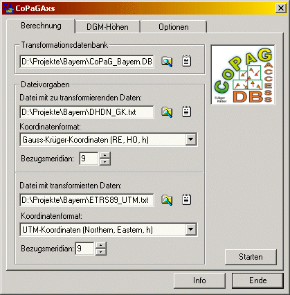
Figure B1: ScreenShot of the CoPaGAxs software at the example of transformation of DHDN positions to ETRS89 positions.
Click to enlarge image.

Figure B2: ScreenShot of the CoPaGAxs softwares options with respect to different features such as the method of residuals interpolation.
Click to enlarge image.
Download CoPaG and CoPaGAxs Flyer for detailed Information (pdf, 915 kB).
CoPaG Concept - Relevance
As concerns the georeferencing of position data in modern data bases, the availability of
GNSS (GPS/GLONASS/GALILEO) related code- and phase-measurement DGNSS-correction data, which
are provided in different ways by different positioning services in and outside Europe - such
as SAPOS and ascos in Germany - leads to the replacement of the classical geodetic reference
systems by GNSS-consistent ITRF-based reference systems.
So the transformation of the old plan position data (B,L)class related to the classical
reference systems to the ITRF/ETRS89 datum (B,L)ITRF becomes urgently necessary.
On the other hand the transformation of ITRF-related GNSS/GPS-positions (B,L,h)
to the classical network datum (B,L)class is of relevance, as long as the ITRF-related
frame (B,L)ITRF is not introduced officially by the responsible state agencies.
Classical plan networks (B,L)class and weak-forms
The problem of so-called weak-forms (fig. 1 left, fig. 2 left) in classical networks has to be considered. E.g. for western Germany the weak form distortions of the classical DHDN network reach an amount up to 2.5 m (fig. 1 left) and for the country of Baden-Württemberg, part of Germany, we have an amount of up to 30 cm (fig. 2 left). These long-waved geometrical distortions of the classical trigonometric networks restrict the evaluation of precise transformation parameters to local areas. E.g. for an accuracy of < 1_cm for transformation parameters an area size of (7 10) km) is typical for the German countries with respect to the DHDN datum.
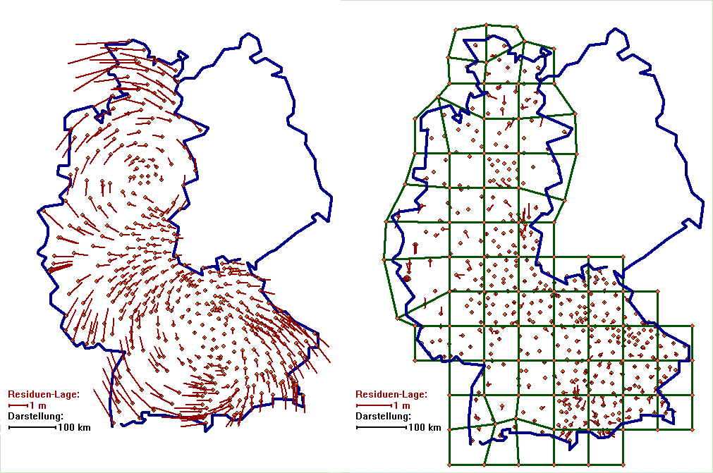
Figure 1: Residuals of the CoPaG-Project for western Germany without patching (left) and with patching (right).
Click to enlarge image.
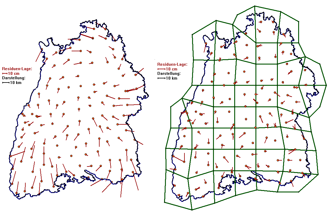
Figure 2: Residuals of the CoPaG-Project for Baden-Württemberg, Germany, without patching (left) and with patching (right).
Click to enlarge image.
Mathematical Concept and CoPaG Software
The transition between the global and GNSS/GPS consistent ITRF-based frame and respective realizations such as ETRS89 and the world-wide existing classical and national classical trigonometric networks is basically related to a 3D similarity transformation. Basically two equivalent models are known in mathematics and geodesy with respect to different parameterizations. The first one is the classical model (type 1) described by three translations tx, ty, ty, three translations ex, ey, ez round the axes of the coordinate system and one scale s. The second one (type 2) is related to only one rotation r round a space axis. Both types may further be expressed equivalently in terms of different coordinate representations e.g. Cartesian coordinates (X,Y,Z) or geographical coordinates. A classical representation of type 1 - implying the seven parameters p=(tx, ty, ty, ex, ey, ez, s) and using the geographical coordinates (B,L,h) is given by the so-called Molodenski approach. In the Molodenski approach of the 3D similarity transformation for the transition from a system 1 to system 2 the formulas read
B2 = B1 + ∆B(p) (1)
L2 = L1 + ∆L(p) (2)
h2 = h1 + ∆h(p) (3)
Transformation Parameter Databases
The respective databases which can be produced by the CoPaG-Software are used both in GIS as well
as online in ascos®/SAPPOS® GNSS-positioning. The so-called
CoPaG databases are used for the strict and continuous 3D-transformation of classical plan networks
to the ITRF/ETRS89 datum (B,L)ITRF in the GIS domain and so-called
DFLBF databases are used in present GNSS-positioning, in order to transform online or in
postprocessing ITRF/ETRS89 positions to the still existing classical plan networks (B,L)class.
The DFLBF and the CoPaG databases conatain essentially
- the meshtopology,
- the meshparameters p,
- the residual information.
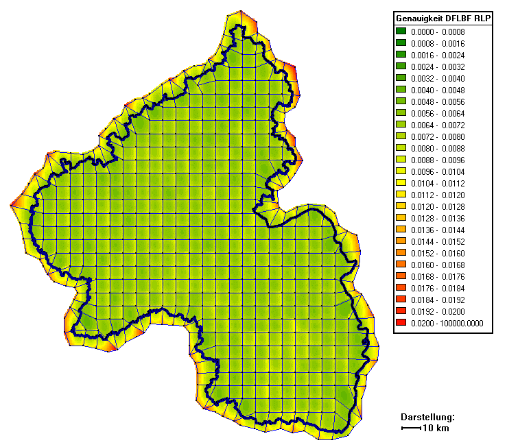
Transformation Parameter Accurcy Surfaces
Applying the law of error-propagation to the adjustment result and parameters p in all meshes, we get with respect to the mathematical model (1), (2), (3) the position (x) dependent accuracy of the different transformation parts. So we for the accuracy of the position ∆B(p), ∆L(p) and height transformation parts ∆h(p)
σ2∆B (x) = σ2∆B (Cp, x) (4)
σ2∆L (x) = σ2∆L (Cp, x) (5)
σ2∆h (x) = σ2∆h (Cp, x) (6)
σ2B2 = σ2B1 + σ2∆B(Cp, x) (7)
σ2L2 = σ2L1 + σ2∆L(Cp, x) (8)
σ2h2 = σ2h1 + σ2∆h(Cp, x) (9)
The transformation results in system 2 and their accuracy σ2B2, σ2L2 and σ2h2 clearly depend both on the accuracy of the transformation parameter databases represented by the parts σ2∆B(Cp ,x) and σ2∆L(Cp , x) for the plan position, and by σ2∆h(Cp , x) for the height, and above this from the accuracy of the coordinate input from system 1, namely σ2B1, σ2L1 and σ2h1.
The examples of the accuracy surfaces (fig. 3 and fig. 4) show, that the database accuracy part is rather high, so that the accuracy of the transformation result in system 2 is more or less dominated by the accuracy of the input system 1.